Tutorials
This page contains a few tutorials explaining the usage of the main functions in UNRAVEL.
Fixel weight maps
Fixel weights maps can be obtained using the unravel.core.get_fixel_weight() function:
import nibabel as nib

t0 = nib.load("peak_file_0.nii.gz").get_fdata()
t1 = nib.load("peak_file_1.nii.gz").get_fdata()

peaks = np.stack((t0,t1),axis=3)

trk = load_tractogram("trk_file.trk", 'same')
trk.to_vox()
trk.to_corner()

fixel_weights = get_fixel_weight(trk, peaks)
Example
A complete example code of the main functions is available in the unravel.example file.
1import os
2import numpy as np
3import nibabel as nib
4import matplotlib.pyplot as plt
5from dipy.io.streamline import load_tractogram
6from unravel.core import (get_fixel_weight, get_microstructure_map,
7 get_weighted_mean, main_fixel_map,
8 plot_streamline_metrics, total_segment_length)
9from unravel.utils import plot_streamline_trajectory, get_streamline_density
10
11
12if __name__ == '__main__':
13
14 os.chdir('../..')
15
16 data_dir = 'data/'
17 sub = 'sampleSubject'
18 trk_file = data_dir+sub+'_cc_bundle_mid_ant.trk'
19 trk = load_tractogram(trk_file, 'same')
20 trk.to_vox()
21 trk.to_corner()
22
23 # Maps and means ----------------------------------------------------------
24
25 peaks = np.stack((nib.load(data_dir+sub+'_mf_peak_f0.nii.gz').get_fdata(),
26 nib.load(data_dir+sub+'_mf_peak_f1.nii.gz').get_fdata()),
27 axis=4)
28
29 fixel_weights = get_fixel_weight(trk, peaks)
30
31 metric_maps = np.stack((nib.load(data_dir+sub+'_mf_fvf_f0.nii.gz').get_fdata(),
32 nib.load(data_dir+sub+'_mf_fvf_f1.nii.gz').get_fdata()),
33 axis=3)
34
35 micro_map = get_microstructure_map(fixel_weights, metric_maps)
36
37 weightedMean, weightedDev = get_weighted_mean(micro_map, fixel_weights)
38
39 # Colors ------------------------------------------------------------------
40
41 fList = np.stack((nib.load(data_dir+sub+'_mf_fvf_f0.nii.gz').get_fdata(),
42 nib.load(data_dir+sub+'_mf_fvf_f1.nii.gz').get_fdata()),
43 axis=3)
44
45 rgb = get_streamline_density(trk, color=True)
46
47 # Total segment length ----------------------------------------------------
48
49 tsl = total_segment_length(fixel_weights)
50
51 # Printing means ----------------------------------------------------------
52
53 print('The fiber volume fraction estimation of '+sub+' in the middle '
54 + 'anterior bundle of the corpus callosum are \n'
55 + 'Weighted mean : '+str(weightedMean)+'\n'
56 + 'Weighted standard deviation : '+str(weightedDev)+'\n')
57
58 # Plotting results --------------------------------------------------------
59
60 slice_num = 71
61
62 background = nib.load(
63 'data/sampleSubject_T1_diffusionSpace.nii.gz').get_fdata()
64 roi = np.where(tsl > 0, .99, 0)
65 non_roi = np.where(tsl == 0, .99, 0)
66 alpha_tsl = tsl[:, slice_num, :]/np.max(tsl)*2
67 alpha_tsl[alpha_tsl > 1] = 1
68
69 fig, axs = plt.subplots(2, 2)
70 axs[0, 0].imshow(np.rot90(background[:, slice_num, :]), cmap='gray')
71 axs[0, 0].imshow(np.rot90(main_fixel_map(fixel_weights)[:, slice_num, :]),
72 cmap='Wistia', alpha=np.rot90(roi[:, slice_num, :]))
73 axs[0, 0].set_title('Most aligned fixel')
74 axs[0, 1].imshow(np.rot90(rgb[:, slice_num, :]))
75 axs[0, 1].imshow(np.rot90(background[:, slice_num, :]), cmap='gray',
76 alpha=np.rot90(non_roi[:, slice_num, :]))
77 axs[0, 1].set_title('Angular weighted \n direction')
78 axs[1, 0].imshow(np.rot90(background[:, slice_num, :]), cmap='gray')
79 axs[1, 0].imshow(np.rot90(roi[:, slice_num, :]), cmap='Wistia',
80 alpha=np.rot90(alpha_tsl))
81 axs[1, 0].set_title('Total segment length')
82 axs[1, 1].imshow(np.rot90(background[:, slice_num, :]), cmap='gray')
83 fvf = axs[1, 1].imshow(np.rot90(micro_map[:, slice_num, :]), cmap='autumn',
84 alpha=np.rot90(roi[:, slice_num, :]))
85 fig.colorbar(fvf, ax=axs[1, 1])
86 axs[1, 1].set_title('Fiber volume fraction \n (axonal density) map')
87
88 # Along streamline metric --------------------------------------------------
89
90 stream_num = 500
91
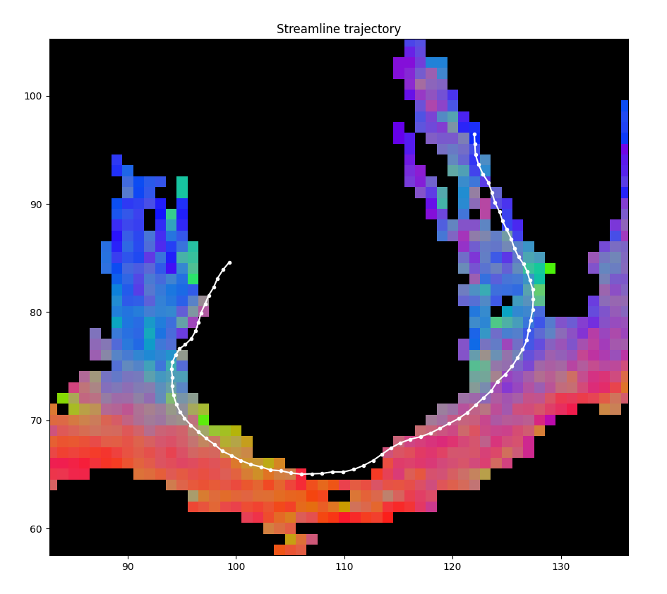
92 plot_streamline_trajectory(trk, resolution_increase=3,
93 streamline_number=stream_num, axis=1)
94
95 plot_streamline_metrics(trk, peaks, metric_maps,
96 method_list=['vol', 'cfo', 'ang'],
97 streamline_number=stream_num, ff=fList)
Adding color to streamline trajectory
The color parameter can be set to True to add directional colors:
plot_streamline_trajectory(trk, resolution_increase=2,
                                        streamline_number=500, axis=1,
                                        color=True, norm_all_voxels=True)
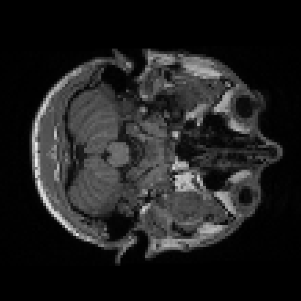
Create GIFs from 3D volumes
Short videos can be created using the unravel.viz.convert_to_gif() function:
import nibabel as nib

rgb = get_streamline_density(trk, resolution_increase = 4, color = True)
t1 = nib.load('path_to/registered_T1.nii.gz').get_fdata()

# rgb = overlap_volumes([rgb, t1], order=0)

convert_to_gif(rgb, output_folder='output/path', transparency=False, keep_frames=False,extension='gif', axis=2)
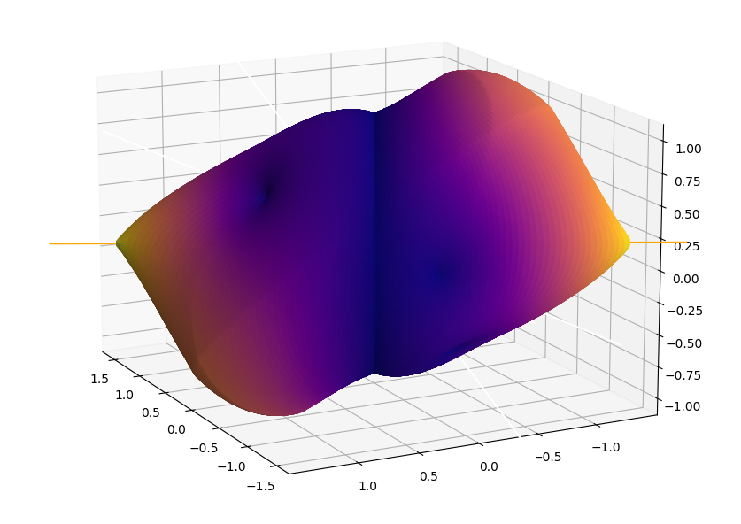
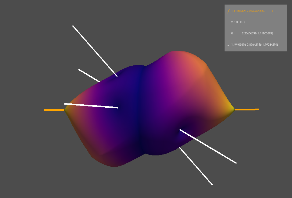
Visualize relative contributions to a streamline segment
3D plots of the relative contributions of k fixels to a streamline segment s can be visualizes for every method using the unravel.viz.plot_alpha_surface_matplotlib() to easily compare the different contributions:
vf = np.array([[1, 2, 0], [1, 0, 0], [0, 2, 1], [5, 3, 6]]).T
vf = vf[np.newaxis, ...]

plot_alpha_surface_matplotlib(vf, show_v=True, method='raw')
plot_alpha_surface_pyvista(vf, show_v=True, method='raw')
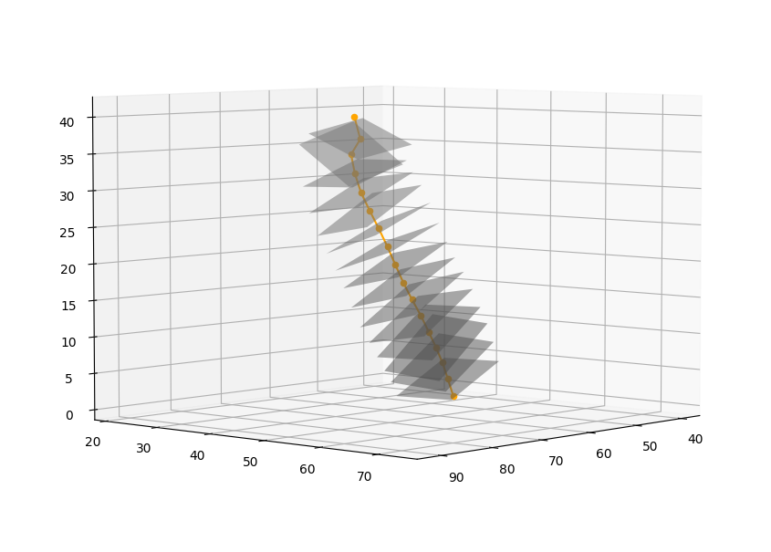
Visualize a streamline average trajectory
The average pathway of a streamline can be computed to analyze the metrics along its pathway or to filter unwanted streamlines. This pathway can be visualized using unravel.viz.plot_nodes_and_surfaces():
point_array = extract_nodes('path_to/streamlines.trk', level=4)
plot_nodes_and_surfaces(point_array)
Note
More tutorials will be added in the near future.